Tag Archives: Max

Teaching Max to play Dance Dance Revolution

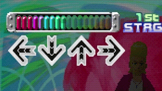
I’ve been playing some old games with OpenEmu recently, and got hooked on the idea of automating DDR game input by reading content from the screen with Max and sending virtual keystrokes back to OpenEmu. Here’s a quick example of what I ended up with:

Max plays some of the more difficult levels of the game.

The backstory…

It all started when I found some PlayStation ‘dance mat’ controllers (like these) that were made for the Dance Dance Revolution PSX game. I have an original PSX and a copy of the game that are boxed up somewhere, so I tracked down an ISO of the game (and connected the mats to the computer with a PSX to USB converter) to try them out with an emulator instead. The mats had been folded up for years and no longer worked very well, but the futile exercise got me thinking about how you might create a virtual DDR-bot with Max that could ‘read’ the arrow information from the screen to trigger button presses automatically.

The idea took several approaches before the system was confident enough to know how to play. But, as it turns out, we can get surprisingly far with some primitive computer vision strategies.

Here’s how I built it…

OpenEmu

Setup

The first thing that is worth doing is making OpenEmu’s emulation larger. The size of the game window (at 1.0x) in OpenEmu is 300×240 (which is a little small on my 2560×1440 display), so I elected to upscale the window in OpenEmu a little bit (2.0x) to make it a little more ‘readable’ on my screen.* As we’re going to use Max to observe the game though, this means that we’re actually asking it to watch 4.0x as many pixels (given that it is doubled in width and height… but my 2013 machine seems to cope OK).

* As well as adjusting the scale of the window, OpenEmu lets you apply filters the emulation, so I’ve kept this as Pixellate to preserve hard edges by duplicating pixels without smoothing. (Nearest Neighbour would also be fine). We’ll re-downscale this in Max with interpolation off (jit.matrix 4 char 300 240 @interp 0) to reduce our pixel crunching.

While the game window is now upscaled to 600×480, the actual location of the game window on my screen starts at (2, 45) given the border of the windows and menu bar in macOS Catalina. We’ll therefore ask Max to watch the desktop with: jit.desktop 4 char 600 480 @rect 2 45 602 525

Getting the Game Screen Into Max

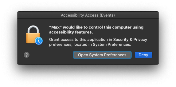
Getting the game screen into Max was fairly easy, but the first time you use jit.desktop you need to explicitly give it permission to capture the screen.

Once the permissions are granted in System Preferences, we are able to capture the game window. Progress.

One of the first things I noticed after doing this is that there are a number of visual cues around the screen which might be helpful to time the simulated keystrokes. One of these was the way that the target arrows pulsed in time with the music.

The monochromatic arrow areas pulsing in time with the music.

At this point, I started working in parallel on being able to trigger OpenEmu from Max.

Triggering Key Presses in OpenEmu

A Major Catch

This part of the process ended up being a little more involved, due to the way that OpenEmu captures keyboard events. The initial plan was to ask Max to trigger keyboard input using something like 11olsen’s 11strokes object. Unfortunately, OpenEmu captures keyboard input events a lot lower than Max can send them, so it won’t respond to AppleEvents or simulated keyboard input.

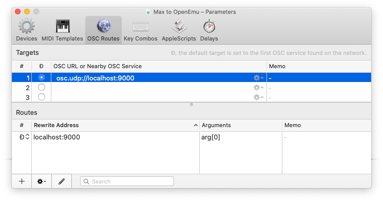
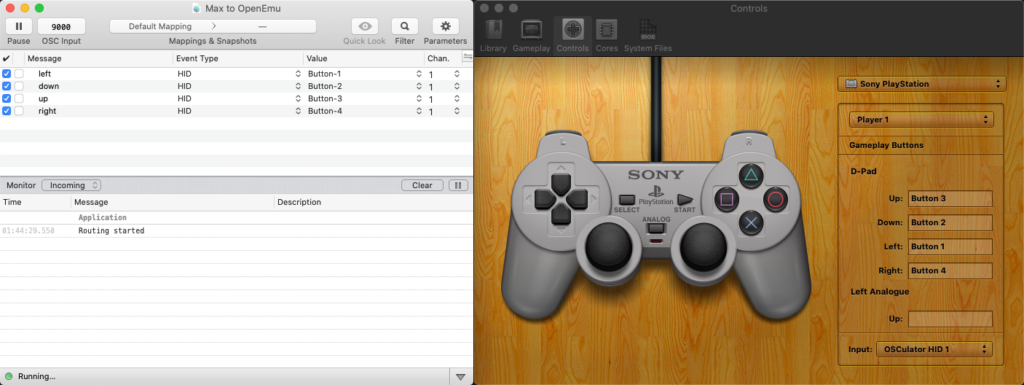
OSCulator-in-the-Middle

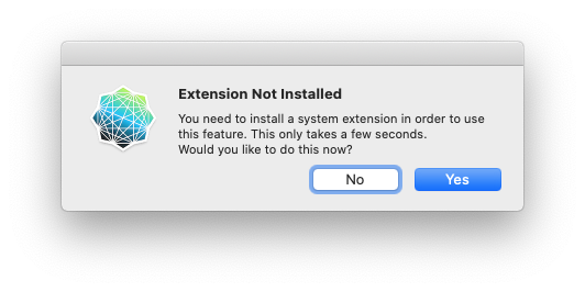
The solution was to creating a virtual joystick with OSCulator, and have Max pipe OSC encoded instructions to it that could be converted to HID events.(See https://github.com/OpenEmu/OpenEmu/issues/1169). To create the virtual joystick, you need to install a system extension.

After installing OSCulator’s Virtual Joystick system extension and setting up the OSC routes, I was able to map OSC messages to HID button events.

OSC encoded inputs in OSCulator are translated to HID output events, which are mapped to Up/Down/Left/Right inputs in OpenEmu.

Crisis averted. Back to the fun stuff.

Identifying Arrows

A key part of having Max play DDR autonomously is that it needs to be able to understand when an arrow passes the target area. Like the pulsing monochrome arrows in the target zone, the rising arrows also have a few characteristics: the centre pulses white, and the arrow shape’s hue rotates through a variety of colours.

As the arrows ascend up the screen, they pulse in time with the track.
When an arrow passes over the target zone, the internal colour inverts to white.

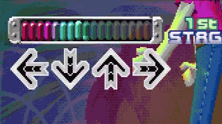
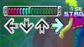
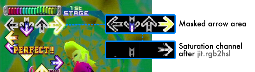
It took a bit of thinking (and a bit of experimenting) about how best to identify arrows as they pass by the target zone. I came up with a series of masks which I thought might help me draw out useful information (and ignore the background area around them).

Centre Zones
Arrowhead Outlines
Arrowhead Shapes (Filled)
Arrow Outlines
Arrow Shapes (Filled) — this is the one I ended up using.

One initial thought was to watch the internal section of the rising arrow and wait until it goes white (using the ‘Centre Zones’ mask below to concentrate on this part of the arrow). This produced some positive results until I noticed in some of the more fast-paced songs that it only pulsed white on quarter-notes… which meant that fast songs with eighth-notes were overlooked. I decided that it might be best to use some of the other masks to try to identify a shift in from monochromatic to colour in the target zone.

Watching the centre section of the arrows turn white is OK for quarter-notes, but eighth-notes pass by unnoticed.

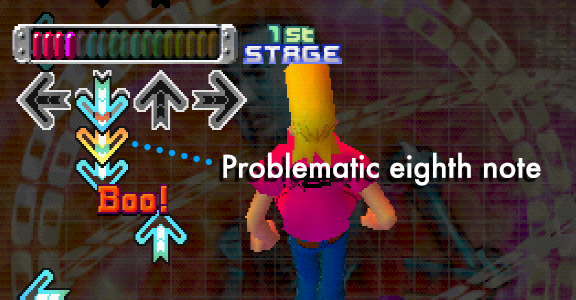
The way I ended up identifying arrows with moderate success was by masking the arrow target areas, and watching for increases in chrominance. Tracking the white parts of the arrows meant that I couldn’t identify notes on off-beats, so switching the approach to identify increases in chrominance as the arrows passed the target should help overcome this obstacle.

The arrows in the target frame are pulsing, but they remain grey (which means that the R, G, B channels are roughly equal). When an arrow event passes through the target area though, it brings colour in to the frame. The amount of colour can be identified by converting the RGB matrix into an HSL matrix (jit.rgb2hsl), then piping the third outlet (saturation) into a jit.3m and watching the ‘mean’ levels of the single channel matrix.

Arrow area is masked, and the result is sent to jit.rgb2hsl to identify deviation from monochrome.

Watching Changes in Chroma

In the bottom right corner of the video, I’ve created a collection of multislider objects to illustrate a running history of how Max understands the arrows as they pass the target area. Note that we have spikes that indicate the highest point of saturation in colour that indicates when the arrows are most aligned with the arrow target areas. While we can use this information to identify when an arrow has aligned with the arrow frame with quite good accuracy, we (unfortunately) determine the peak value when the arrow moves away from the target area, which would mean that we would trigger the events too late. Perhaps a different approach would be to ask Max to trigger an event when it crosses a threshold, and use this downturn event to reset the state with a onebang (allowing arrows to be triggered again).

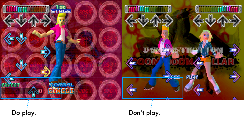
Limiting Input to Songs Only

So that I didn’t have to juggle with starting and stopping Max from acting when it shouldn’t, one of the final touches I added was to disable arrow triggers if part of the game screen wasn’t in view. (This is why you might noticed Max go to sleep in between tracks.) Max will watch the score part of the screen to understand when to trigger arrow events. This ensures that arrows are not triggered on Demonstration screens, or other spurious instances of colour in the masked areas.

We know that a song is playing when two features are on the screen. The frame around the successbar and the border on the score.

Future Improvements

The video at the start of this post shows an example of Max playing some of the more difficult tracks in the game:

  • “If You Were Here” — Jennifer. [Paramount 🦶🦶🦶🦶🦶🦶🦶]
  • “Afronova” — Re-Venge. [Catastrophic 🦶🦶🦶🦶🦶🦶🦶🦶🦶]
  • “Dynamie Rave” — Naoki. [Catastrophic 🦶🦶🦶🦶🦶🦶🦶🦶🦶]

As can be seen, there are occasions where the timing of the triggered arrow events is not quite right. The system completes “If You Were Here” and “Dynamite Rave” fairly well, but struggles a bit with “Afronova”. This is mostly due to limitations in my implementation: as I’m purely using the screen to identify the events, the system gets easily fooled by rapid repeats when it can’t discern a drop in colour between frames.

Alternative Approaches

There might be some creative ways to get Max to follow the BPM of the track a little more acutely (and therefore quantize arrow trigger events) by performing some kind of beat detection on the music track. Alternatively, we might be able to determine the BPM of the track by watching the rate at which the target arrows pulse. Instead of just watching the arrows when they enter the frame, maybe it might be more robust to measure the optical flow of the rising arrows and time their triggers with a sub-frame temporal accuracy.

The Patcher

There are a couple of other things going on in the patcher if you want to download and have a snoop around. (Of course, you’ll need to do some setup with OpenEmu and OSCulator.)

Synthesising the THX Deep Note with Max and MC objects

The addition of MC to Max 8 added some handy ways to organise audio signals. One of the simplest benefits is the ability to pack stereo channels together with mc.pack~ 2 and process each of the channels with only half of the number of objects taking up space in your patcher (filtering stereo signals would previously require multiple biquad~ objects for example). MC also opens up some helpful ways to think about additive synthesis voices, richness of sound, and polyphony, and simplifies the patching needed to realise certain kinds of synthesised sounds.

One thing that is really wonderful about MC is the simplicity in which synthesised sounds can be made richer and fuller in the stereo space by modifying a group of oscillators’ frequencies and panning the individual ‘voices’.

Many softsynths — such as Native Instruments’ FM-8 — offer the ability to add more voices to ‘fatten up’ a sound.  The addition of extra oscillators combined with a small amount of detune adds a fullness to the sound that — before MC came along — would have required a fair amount of patching to replicate in Max. With MC objects though, this can be accomplished quite simply with MC object messages like ‘deviate’ and ‘spread’ eg. deviate 0.1 0 (to produce random bias values ranging between -0.1 to 0.1 for each voice of an oscillator) and spread 0. 1. (sent to the right inlet of mc.phasor~ to evenly spread the phase of a series of control oscillators, for example). Using these messages with objects like mc.sig~ can be useful ways to widen MC signals within the stereo space when mixing them to stereo with mc.stereo~ (or mc.mixdown~ 2).

Synthesising THX Deep Note using MC

Several years ago, on the 35th anniversary of its first screening, THX Ltd. released James A. Moorer’s score for the ‘THX Logo Theme’. Commonly referred to as the THX ‘Deep Note’ the theme is an instantly recognisable musical motif of swirling noise that coalesces into a D Major chord spanning 5 octaves.

The score describes the THX Logo Theme as thirty voices at random pitches between 200Hz and 400Hz.  Each voice moves slowly and randomly for a short time before proceeding to a predefined target note. The idea lends itself beautifully to MC. [Source: https://www.facebook.com/thxltd/photos/a.379994786929/10155235575876930/]

Building the THX Deep Note in Max is a great conceptual exercise, and drawing on the MC approach of thinking makes producing something like this quite straightforward. Here’s an example of how it might be done.

How does the patch work?

  1. An mc.sig~ object is given 30 voices all of MIDI pitch 61 (or C#3).
  2. These are scaled to the range 55–67 by an mc.rand~ object that outputs 30 randomly varying values — constantly shifting the incoming values from mc.sig~ up/down by an amount of up to 6 semitones.
  3. At the same time, 30 voices — the final chord, comprising 10 distinct pitches of 3 notes per pitch — are being broadcast by another mc.sig~ object.
  4. The two competing mc.sig~ values can be interpolated between by using the mix operator in a mc.gen~ object.
  5. The MIDI pitches are translated to frequencies with mc.mtof~. Keeping this as MIDI note numbers up until now is kind of nice as it allows you to think about things like detuning and pitch shifting in ‘cents’, due to the linear nature of pitch intervals in MIDI.
  6. Adjusting the main ‘Deep Note controls’ slider lets you play with the transition at step 4 in realtime. The values output by this slider object are fed into the Transition to pitch, Amplitude swell, and Pan function objects, which means that the different aspects of the sound can be independently styled while keeping the controls simple. The slider fades the sound out at either end, but bringing it in on the left side introduces the dissonant swirling noise, and dragging to the right starts the transition to ‘consonance’.
  7. The pitches produced during the transition are drawn on a stave with the nslider object, and an mc.scope~ shows the inter-pitch deviation.
  8. The sound is mixed to stereo with an mc.stereo~ object, where the placement of the different voices are subtly distributed in the stereo space by an mc.sig~ object that outputs 30 random values between 0.25 and 0.75 (due to the deviate 0.25 0.5 message).
  9. A few objects are used to roughen up the sound a little bit and boost the frequencies in the low end.

Here’s the patch if you want to have a play around:


----------begin_max5_patcher----------
5396.3oc08jsbqabkOq6WAJUoJmEck68kLujTwSVdvYbEmopoJeccKPhVjvF
DfF.T5JmJp7+v7CjmxGx7o3ujo2.3hHAa.BQJoKuhhMZftOq84b5Se3+3cWc
8jhOoptN52F8MQWc0+3cWcksISCW4+7UWuH9SSyhqrc65b0CES9tquwcoZ0m
psMWGAaZaYb8z4o4y9XoZZs6QCw.9sfahHX1sH5MQHj4SleG8s96Je0hz7LU
scTf9FSSrOb8.9dHPb85tVrpd295Zp9wkJ2XdcZtdz+VyE+mu6clecyoAhUp
rNARoEDobKrgIcCgn8Agr8CgnCAgShymc8MQWOpfYR0xp53Z0SGGTIfa0DSF
b.DS59AURWDSMjdWVQr8O7edvz3oEKVnLOicf9+97zpnGRyxhtKsTE8vbUdz
W70eUjtUUd7jLUxMQSVUGkdWTwRUtFsDcWYwhnoYoKmTDWlnu4541aINqTEm
7XT4pbS+tI5whUel9AmqTIQ0E5mW0J8PTOOtN593xzhUUQZjiFIWEEquPZdZ
cZbVZkJ41l4YVZtZZwpb6jk1AAxRSX.pSbCZ+HWzKRDY+jHfu0IqlnQG16d.
3eMNrtHuCVLrULhAYFVLJwwu0q4OX8SuLdgpVU9QGIbSnHPcIVIsAwnsJPHE
CcjJfkTgw8.TkhPfz4w4IE2cm8t5ovWidlV8Mmhj2BUUU7L0yj79O9PoteQY
wqxmNeRYwCUpxn400Kq9se9m+IL+9a0xr1+3y086yqm+o2mnTKeedQs58ZX6
8KltWoDxwv7HA07Fjhsbb8Qksj28ZRySSRT4cxYMtpufctJrDKsPpV8MludY
XPe30NlVgYSKxJJcCnd4ADkHAPICvEDL7FcShM9LliLMIITfT.vRDjxDL8Lz
LiFSzBnKzBhaQKDFeSiS5EVA+VDqH6Bo3EGf5ofEq.k8GqfdKhUDAgUPvAiU
fuEwJ7tvJ.lvt9LkMXjB3sHRg0ARQf8qp.FJNQHeKhSnAH9v.ClQQHdKhTHA
fTzqHOXjB+sHRA2ERghstXhzhO7AhTXuEQJn.3TPrgyoPeSZ9VmHEB0oSwYZ
auQI72j7I+w3DUjd1FEWGMonddjJOopKzDg6Vila8uDhn8GQcHCWFuXOUFMs
HutrHqSPAKvV9eJlYAIQ2weB7bPgw5YrDG2.IFDTxcx5P1Zt6dEiMF8EmbsX
5sYoKRepSwSGeGD5.AuFrdAHjdRrVrJqNc5737bUVU5r73rgQ9tKMqVUNqLd
47NAQjz4VMf5cfjxbxXaFusrz7EwkeuprpQShEq.bBhPlYAOZauuSyfbW7zc
CU0Z7jXO3Ib+C3EuY1ULaOyNPyasuuo9hmg2yRq1NHsc7GM80EFol4lCiuE0
sRU6Z0OwzrP5oxMl+viiYDf.KXHLfvDFiEH2xfDDU+Yh95DnvnQlpUHyXRt.
vwPqNZvA+0XJrqkQlj9CqhSBSJwE7AsRZZWRIr8P8QWHojNzMTTppdRq6B.h
.g.8.gWP5H6n.94fOkeg.+CENSPDF.5DpIThUcQST5c1wzqsLhdYWGaYVZsQ
dAZr3QJCZMatUHSB5MElH54tisiRmQ07quPoVF8WKpUlMFpZdb4xnIOFEOwX
QFEDMUeOU6eSaPcsPBwsOGLoyoGHs26E.AOdq5eHf+uopJxVUmVjGMcdQYRj
ID7cZKCS31oPerPvvda7IVdNrl427jYkh.TUQ8NqyP8VlEeozTcHx4+0hz5p
n4oylG8EQZZ5WVn0aW9YZ95o5+HJNOIJMupVEmDEmjToaP6ugpL59hzoJyFY
p8+ntXQT87RkJZhd3bLD212siQaxK2vlXr6vx+6zUv5CeBj9xy++Uw4QyT4p
x3rrGMH.M5vJxWpbaNrFMEEGoUNpG9nIZcjE2EoQfkphnpklMEduXFbWqU.s
LZBlOryTKlgv6Clg7xiY94e5e++8uLP+xX6ddqA93JCFZQw8JKZZVYwpkZ9o
03CiUt8UQI14ymT3CDBi0aEkPvYvaV8BOItMM83oFCv47.i1auYg3yhU.Gbs
vx3GbR7FsGU0w2q5bs.oUHmhjNZGTz6ECfnywhAIJsqeIpmhfQPTPlu58+CB
X815F1qKq2KiVj9oNgYjirIcf7wR2o8v0RunLse3ZLvsBVkIDZkljiXQzxTM
jpaYhp9AkJWyUB9y+ncEPh4u9v0QeyS+IzO+S+u+I721ac39vDvDtE2FfJ7y
fF70F1taLpBV4LE4bkUdKai0pX8I4cZUn4RxnpzD0lX28GnVSLSpR+QaOQF9
wmkmRa.re2pp5z6RmFaLi0dGCw2uo2p9wj3oOc7r6Q3PJHb6agqs6EWYWkVR
Ha0htTaigVpn.37Pg26n3gfzyvBtZ6N5bsVry6SpyLJLq2ZsPPxkMzwcCgdx
DzupJVL.5D9Lvu08pKdnfHrrYGiJsWf.cFTUlVUUjGmOM.4FWNx5BouIIrZg
Dm1okEoN8pfaAAChv8qjD8Bl0lGBU7GJxONpf4W+i1jKpciJf8.U.N+nhwvl
eAkZsEX.17i.xKp8SM6+XWY.iKV1NfiJFQV+0GEfKOq+u7qmFqmAQZaALFQ9
zmUEkntO0ZWg1OWsuue4e4K9KV+ihnz2y3FaMmo9U21e6GcooX6t+6Tt2KCH
QG5HF.FwHeq00g6LFZHOigKZftbRsWgPCAfWXmG94e5eGohmN2GDLS3Mphpx
JdH6Qq6BN+Ixd7CW2+Xa3rQAtcnd5WrMNTdIOp1ZcLO8EBWXdYt3aLf3ZHoW
nzq9f1sb7navrGXAI.adize6jgRxKNsqNJKZZlJtL.HQ3bfYPPBtm6XiYyZb
yqwjpsrTsTokIs6UQHPrigUvF.DitjNGDlsG9cfyGFhgDtQI70OT5WiAp4dG
LXBtrd5E.X5jM4.OPN.YTwK+9pELb3OOgTw..i9d3PG9A55PFE7WsQ.2jWKp
j8rMZ+xz7oYqRLaJBpIviKUkNCCSysaNhYuy9U81tPtFgYLTPfuU311LR+2b
HA+Ux1g3ClNhN3cCQbYir7eWa6WUp07esw+1HJ2A7Rg1cCg3OCZ.b+2LDwYH
rv+m17H6ySRqLuq8vodUtp6Hsw17LUocdo+.FWLd.VcwrYYpP1GNu6UH2NZz
qibJmMhG4zw93qqcPcl4Xca1NqPvCMm6KT+8OSqA5BscVGmL6MxqY6GGDYF+
ZfLeH2uiWtL6w6iyVoWfQHadwZdA8u3D+Klr4Ex+hxadA7uHTyKrv7Bwzu5c
pcPkN6w3L2QOU2PuOssP9E0vy5nIQSBf0p4zMQFfCDGJosQAczrGFzVkklnJ
Oti7XfiDJcYcOTdLR2hhD0ASSmVVn6197UrSt3tNknCWVCs+StgXiCjAxvCF
ZScjxymZYnPaa3x0UZiz73o0o2qhyVNOd6XfuOxhlPP.x0+ShVSjf3mSjlFm
MsUXk0HsNqLMYK7Dlr04Y4lfa5HrC13d5s54VhaGhIfM+g09.1hUAb.VEh.g
05wIZaFYDt8n3DRSvsmnG+H+XyV70+ZyHXeWyFNyHm2JvRixFhzmDwCnHrvv
W3hvxAf+ePKlWVDA6N8oaVHm4rSgM.yT5cNyeBZY2OnZL4Y1QRWJajD4PgyO
g9SloGvEebWgg6EhztLd52GBzRo1HwMfhnD8xFBN8iW4bu+5i6xtmndr31rW
vDNfXqN1fZdRzuKWEWppNR4+xSVYBrK+d6+Ic.RjWR55Ol4ybUVH5j3ZkxVv
c.fo3RSW09IVkGurZdQ8SgPSIhgJpRNe7vGxYoeAzjiegbvUNgSoCr2o7+nR
PM9n8TPfHNrj4bufXeqccdu7u4EXQU6A4HfPbzj93Dz.fW5k5PotJepMmEOZ
NGgbtBP8IXMeSWARJVDmlusKFFGAppUK+3mboiALTCLvj9GODxQO0VM+2ydz
DvA0LUdxlO23jDaNjT8LOHuY2OfvPgf.nbIGBfDqaLRp.u9GeGoX1l80zDWJ
Xv0+36HmnwxZWFoT.GQX1i9OUKP09iz2QgT6LY6S0UP.bmf0aa903Vf.LYnf
4jX.8mFsOKff1R7EBKfOze39Wj.fX74H27+0gbZZYbrufdQZKrW8PBG9p6.0
9qMGOsNMzh.29vj.5ulMD6UGb+aBgZS8qdAICvrKzkRc9QC9VSF8Bbwq1qMW
atEecnw997hIUyicStlpBZSjIBOOJgHzvCrsUust8kqpOia11W0Y1PSc0MTs
5ZWR3CFvIMZDy99vW5V3NgruLKcuQb3ducC22LJqaA6fWaqqqmu.6gJwsrNh
xjZ+PjL.gSv1lfLAEKwHpff3M8iZJ4CHJRxHtVuEBP5aCQILAT6AiuiP.fKA
l0uwXazT0MA0F.voHAPuJunsiDABos6AK3Xpq9R.HZqJgPFDPDr1k8gTgdn3
Ll17ABTZg.nuK5ggxYsOxFv.Hv..w1SDTpsSAhvTo1.CViUL7M+G10ShDvvL
Nf.gZqQ78DuwXKjb2nKYLjzL40LYjlmYCnv4BFkYM3A.jXFFosOR.fsOQNkH
IF.kvPDWzwoaB4M.tGNzlWYHRnN5HGgwHfGQ4hiLPOEZP6s8SpwDZDFGvo.o
zyKP23Y1zSJBxwZrqlhP3BG9QKGyQHAQy..ksz6s3KXdpyFHG.qgEpEGZmrn
NniBDCngNJyMM7yyM4hjqs6686gicT0O96WXpQCqRTQe8CprrtzU5RXJgq1a
HI8WUITdITURck7qWdubf7Wed4rEGHugEDroVQfvoGhiAXrV3QKeCa3pgOyK
Gz1+zH0qYb0pBz5VzRDFsXFkPXsaBHrjqEx4MpGHBAjfzRPVoUoSigaLcb4M
NXwVKJatEqv39z2vATJVq9iIvboSeCiq0QiXMBzMhc7sD7rNhYzmz9iXT715
PwQxkx+JChgZvCgjZhLlMq8jCHZKvySPtCDZogbTWDtMEeHP6Y5ntDTBULF4
QQapTzjMECJgJ3s0nqAmOEfKZbIMAZNc1SQ+NiaTUZqyCHqkaqGnPx.9Rm.+
pyyV6QFxZ.dPXATSsIm3vBj9WM8DjWcHAKWPv3flf2BaBRU+4DDu9XDbkCEs
vP7p5hYZqV5dC0ZK4DM0g7ADzCwkphwExwlecEwSt49tX9c3j4Qz2caot7d0
sFRS67993xbskfGtCc.XbnSSFxWbEM4Ka3PVmdlC6zVTMHU6IhqSubPOn4dK
V2tTN1N0qhuWk7w355xzIqpUq+qJO10idMXO8RpE20zbS6aBSYE4y5DCuUuW
noX1bwowX+ctpyUf2yA685UyKJqCevZvQ66QsJOstp9QG0f3ttkeq4sQSswh
5h6BJT39bRb.msBt70mxx3GBBnwtkHnrdqajKdaFD7l5wCC2ePl+Zb+NXgXN
jOk8o8e2NtXIp9gO7zAIM61OK4s8cWs3f2LV76gUOC8PL3mBdkQbWj9oneAL
fxpk4Lfar4o+NKSnWXB7LUtl.eri8TC0s4K8BBD1ePcT1f1lPEFWGuqAJ14s
qvSusAJ2klotWUV4KcTvVS.hWtbi1uZq6xfA+NWREKtYcao4t1vqaqTce5yd
15GdoFKVqQgqJc1n7o1JidS11WluJss.WXopsSMKsyXdiqhK5yyXC4Zs0MaD
MXegXl3T23JGOzMBGrMKoyJl98pjssBx8sh3xRUkJuts5Zs95Ip6h0zgOtY0
5xt8b6qC6TBz24psFq86KSiyVCFlP7VjalHaScrg90OjlPJ3994YKXx1k73k
6618e2LdfqZxX6UUShKMzNug3n1qVWTjs80VemYp6p8WeYpl2bGDZcwxNtZY
5r4cc2tZyZmOd6kpzFs5t7GMNH7QiY76zw3rLuX+NivmhySWDWqpSczCsKMs
W04Ux7pokEYYaC2tKc+9tjI.iSUOjlTOeqRCi8R5aHcYCi00qI6IoyTU06zX
c7rpcZp0x7Maa0Duz9GqUKVloglc5gV5Q6mi1IgGp78rg8aKTw5uLc2V3eSE
p6bkN2Jmq1VA6+ckqLpZVIQyCVFWWTZq.sqOzoM0tvDe4op1VPRl5qPS0M03
va2Z.1WXGu5fJuENaMcaRcS88aKkCGZ44qdlmrWuysrqe5a57zUMKQMTb6VK
asCpU2qEKi.swc4vfuCf8Ab8Yqa0Cfm2Avu08bnUsOaHmux3a6FUssigbbVq
wXAfb.G.4vdyfbB.s3cMwKw.kAfWvG.uPeyfW1HHlGAw3MtWbBrKv2RnEzQE
i.iEdA8lAuX9tSHP9Er6HyfomfxWRuW4YC6DMqWdvU5sSaSONDJopXU4zFzr
WWWzNvf1Nm5z7VCn+l1ULZ145fnK8epvCcpn0CEgdQmJzPmJjWbrBrOXkW1o
BpOSE3AlJMM2FUZuavOTpcg0EA6eXk56UO59NLmnMoGfwB30iYgR4O++Dstb
S+PZ87nu7OD48x51Oj27c98MQ+Q0jxUwkOZNRCn9VP8N4ud0IA7MEf8gssVA
GpYW5qGA8bFLylSGsQpKseFc3ZZ5ynBgOT7.Fp1IzINVx.FKwnLTPTHCEYTF
pPvf1Jd8oOVlrvMfwZTPgnPPg6B8EkItfjAOGC9Nni1AGbNFbLY+CN5DGbVH
CtYuJNcgeLLDoDvXvMsC15PbtnQYrng.VnQACFD0BOJppwAoptYFcZiEIDNC
64vdjFK3wFKJbTFKQHvkbTTfRBY4NaEY3zGKZPzK5nvySCR8XCl9DGKYvv0I
OVrffK1nrPNCGjV9QgOjQCQ9h.Gsw5LwavgmOSW4AQuXiBeHmDjsOzwPVlGt
0FmLbIBg2fOJVaHAAY65nPtjgwFxGkwJHUTxQgbIChkWhFswBdlfqfTQQ2Vv
XipK+IM51usBN5nSGCg.TPta25T9oMVvfzYgGCcVgYZJZLVllPCMNLm5HQCQ
gEeLzgvAmKFvfVGyBSmJKAmetnSbQv96cpCk.DpWrm7HgCV38jGpvrsYakuK
R257NBMacpsb8ZqrVPBh09wwNVPAMe4jWhXfEjtmwIphgshH3PqHN1Q.KLeH
fgNcNQNfPL4ZLh4BOjkq4igmSAEHIt7rwZgeQhgLkc1BWl0e1iY9JczFoiCT
iggBAEhhQwi2fB7BaLL9mEh5bA7rs8I6DtjVNe7oAkgv4OJwfIjAhNFLiT94
hYTFhDlj+h3cn8qtl.bYaThQBHnXjHFkkA.AsjNXT15B.6LhCChdwGE3JHiz
AOWp1kNB6bZDLixNmAgcN9AO+jGb3Ccvtm2.aJjruSYfI4Pd2+7c++DAEIoB
-----------end_max5_patcher-----------

For fun, try disabling the ‘Enable/disabled detune’ (step 10) to hear the difference between strictly tuned notes, and Moorer’s subtle detuning. The detuning makes it sound more rich and organic. Also, try changing the final resolution chord to match Moorer’s score (step 11). [Interestingly, the score depicts a high 89 / F5 which seems to not be present in the theme itself.]

There’s a lot of nuance to the THX Deep Note, and the end result made with Max here is similar to the original, but there are still some subtle differences. Aspects described in the score (such as how “each note moves slowly and randomly”) sounds a little more like sinusoidal oscillations in pitch in the theme (as opposed to the way they are shifted randomly by mc.rand~ in the Max version here). Rethinking the way they move randomly might be a fun exercise using mc.cycle~. There’s also a non-linear ascent to the final chord in the original which sounds like an acceleration towards resolution. Playing around with the function objects controlling the ‘transition to pitch’, ‘amplitude swell’, and ‘pan’ might be good places to start experimenting.

Links:

Tathagata

The base-chords and note progression that forms Tathagata is something that must have been going through Fredrik Thordendal’s head for some time.  This progression is something that has emerged at least 3 times in both Meshuggah and Fredrik’s solo work, and can be heard as the basis of Tathagata (Sol Niger Within, 1997; Sol Niger Within version 3.33, 1999), the close [3:50] of Sublevels (Destroy Erase Improve, 1995) and the outro [9:06] of Fredrik’s Secrets of the Unknown demo.

Tathagata is a beautiful track that seems to will the listener into innately feeling or predicting the next series of notes.  I was wondering why I felt this way about the track, until I sat down and started to score out the notes.  What emerged was a pattern, or a recursive, self-pitch-clipping algorithm.  (While it is a progression that continues to spiral upward, it has octave subtraction protection to stop it going on infinitely upward).  This is a very cool progression that, while it isn’t an auditory illusion, for some reason makes me think of a Shepard-Risset glissando, Risset’s rhythmic accelerando auditory illusion, or Autechre’s Fold4,Wrap5 (LP5, 1998).

At first, I thought the track progressed in measures of 5, with the notes being played on the 1, 2 and 3. Sarah argues that each measure is divided into 16ths with stresses on 1, 4 and 7, which I now think is actually correct.

In lay terms, the track can be represented as such:

The pattern progresses in a count of 16.

The ‘root’ note starts at MIDI pitch 56, and adds 5 semitones after each loop.  If ‘root’ exceeds 62 (or the initial ‘root’ value + 6), then subtract 12.

‘root’ plays a chord (root, root + 7, root + 12 [they are transposed down an octave in the code below]) on the 1 that rings out over the course of the measure.

‘note[1-3]’ is the melodic progression of the plucked parts.  They play on positions 1, 4, and 7 respectively of the measure.

note[1] = root + 2

note[2] = root + 3

note[3] = root + 11

One possible implementation of Tathagata for JS in Max


// Simple representation of pitches and key modulation in Fredrik Thordendal's Tathagata.
// Tathagata.js by Alex Mesker / alex@x37v.com / www.x37v.com
// Save as Tathagata.js and put it in your Max search path.
outlets = 2;
setoutletassist(0, "Melodic progression (MIDI pitch)");
setoutletassist(1, "Root chord note/s (MIDI pitch)");
var root = 56;
var cutoff = root + 6;
function msg_int(i) {
if (i==1) {
outlet(1, root-12);
outlet(1, root-5);
outlet(1, root);
outlet(0, root+14);
} else if (i==4) {
outlet(0, root+15);
} else if (i==7) {
outlet(0, root+23);
root += 5;
if (root > cutoff) {
root -= 12;
}
}
}

Save the above JavaScript as Tathagata.js and put it in your Max search path.

A Max patch that uses it can be downloaded here:

 ----------begin_max5_patcher----------
1034.3oc0YtzbaBCDG+r8mBMb1MC5EO5jKc54dqSuzloCATrIEPd.4ooMS9t
WP.wOBTDBaYxgPRDfz+8m1c0hzyKWXcO+IVgE3ifuCVr34kKVHappgEM++Bq
zfmBSBJjOlUJqnHXMyZU88DrmDx1QXZaaayYErLQfHlm8ybVnnt+gT3M1q.X
mpq1MW.207RY6RiyRXB4nfZ6o.Q3l3r0G0KxWkhj8E5F5J.z639guSz1QvlV
iijhje+ie.ha04C7LQVPJSdqOkGGjzdm5dP7msr5A0x509u5kJh+q7FvRQT0
5KKWVcYkhHLjmlVxm2fvuvR3Qwg+H6a73vWIbRbFKjuKSbDX5FwXBsBKHj2v
LF1OiadeHVNgQIRTS5Ex1c.Y3vP9BRxOugmGoBGUkHXa3ADg3Odh3YDfjw9c
4f8Fdb6s.h0HCzv1R+GBQ9Kbsik8XhzvtZDoEWMAc2EmH4fhsLVTmPwdXnXK
CPpSnMRn3bsS+zCQJ9ODANX9XnsqjH3AHRGQF6W33hFZz6BWtiMx.gHSaIHL
7Z6CzKL7GML7mHL1Ojyr.hDdPz8AYqsF8pmRh.kIGbrGeJBjN4MkJ8rRkco2
yx0z3cqyFLjwi5v3oZtnwpKAC51yX65Ji..0LwQStRG33yUhbLSYD5M26O04
dx6l4djl4ImxbO7ZVBYZvuXYbAqracAXWpcm..2O.7jqPPbq+zBn63cOf5rR
wCkowkNH0+gA7PlLoP1SGUtuKPUEl5OZZXDQgd5FMActlQSsFNTunHJjpscS
ul1cAKAXO1Tmv5O9D5Q1u+QiKbfpaAUqN2kZVjDG0yJqnAc2QT4FO3ViCeuw
f.xPKfdzGdmxipMSyYidS1DQlyD0p9nZKrwMVq5iPyo5iNhAkDHNcWpr+bza
KDlPci1y+5Fka8HKGXCff8q8bDhnC55Tu8t9dCfHRGo8m.hZ+4bu0bB950IL
8hhH0AQdsWU+qq8GXqGOiEBxD4bvAGLx3RE19oBZryqyiMPnap7XA3qAhMAq
CDA27XgdS+HjrzGOMJMVqi+Ykg1+svDVf1UGfP6SfNt8f6hsmzxmQdzKmbHi
Rynp8igTAeWdX6HztWXf8VRDqPDmIO1qCdnpiz6fGZSbTDK6v5eSii1xKCua
DQOA4ppoSFtt0T0ZRFTSUkFLnlLKl7UPQtFUQJ4KY34MaEoDzbt2pHoS72tz
ZRoHNiqH3.JhXTE4n.ileJxryZTETjiYWLoJZCMfjnFURDURSZ1L2PkRc6Xd
MAUQSlK2MRk4tpCRvjbRkBAfTyqInJZxfycpjbBYVebUpp7j42KtjTIU.ZFp
IrYC6NY35gSlMrCoRp.DY9UAN1rbBqRkSXytDL1U0xBPyLM4OAMU9Our7ez3
5PsB
-----------end_max5_patcher-----------

Pitched Synthesis with Noise Driven Feedback Delay Lines

The other day I was listening to Autechre’s Quaristice and thinking about my first perceptions of the album.  I remember thinking “This album has a very physical-modeling feel to it”.   I had forgotten about this, and recently I was playing around with Karplus-Strong string-modelling synthesis, after reading about the methodology behind it.

The opening of Autechre’s 90101-5l-l has these gorgeous rich resonating tones, which I accidentally seemed to be able to replicate with a Karplus-Strong model.  It sounds like they are capturing an incoming audio stream and then thrusting a noise-grain into a Karplus-Strong algorithm. (There’s more going on in there, but this seems to be the basis.)

Autechre – 90101-5l-l (Quaristsice)

Example of Noise-Grain Feedback using Karplus Strong Plucked String Synthesis Methods
 

In simple terms, Karplus-Strong tones are generated by taking a burst of noise, and creating a feedback loop that repeatedly lowpass-filters the noise and scales the volume back slightly.

The combination of each of these factors plays a part in the resulting tone:

  • The brighter the burst of noise, the brighter the attack and note.
  • The loop time determines the pitch (shorter = higher, longer = lower)
  • The amount of filtering determines the length and life of the note.

Kind of like concatenative synthesis with a recursive function applied to each grain.

So, for fun I was trying to make a synth that would generate tones using this noise-based feedback model using Max.

In order to generate a specific tones, I was basing my pitches on the relationship:

F0 = FS / Z-L

That is, the fundamental frequency (F0) is determined by the sample rate (FS) divided by the length of the delay line in samples (Z-L).  Put simply, the number of times the delay line is read through per second is its frequency in Hz.

My first versions suffered from a very strange thing where the pitch accuracy was shockingly bad.  I was getting weird results where tones were getting more out of tune the higher they went.

The first problem is that I was using a [delay~] delay line with integer sample-length delays.  Who would have thought that something that was ‘sample accurate’ could be a bad thing?

I realised later that it was bad because the generated tones were inversely proportional to the sample rate and that the values were being truncated to integer lengths.  When the length of the delay was long, the pitch was moderately accurate.  However, as the sample length got shorter, the pitch went way out.

The reason why this is bad is quite interesting.  Consider that we are working at a sampling rate of 44100 Hz.

What tone will be generated if we use a delay line consisting of 5 samples?

44100 / 5 = 8820Hz

What about a delay line of 4 samples?

44100 / 4 = 11025Hz

This is a big problem.  As the frequency that we are trying to generate gets higher, the less range we have in discrete tones.

At first, this appeared to be a sample rate issue.  If we increase the sample rate we should be able to get finer tone control.  However, doubling it means that we can get only one new pitch between the two we got at 44100.

88200 / 9 = 9800Hz

This is still not that good.  My solution was to make an abstraction and try some ridiculous upsampling with [poly~].  With this, understandably came a hit to my CPU.  The solution was still not all that good, as only one single new pitch could be attained between the previously possible tones each time the sampling was doubled.

This had been puzzling me for about a week until I decided to drop [delay~] for [tapin~].  Amazingly,  [tapin~] allows fractional sample length delays, as it does subsample interpolation when given a signal as its delay time.

The following is an example of the nature of the low-pass roll-off effect.  The clip starts with a fairly moderate low-pass filter (centred around 1500Hz) that is slowly opened up until it is barely filtering the delay line.  As the filter starts out strongly attenuating, the note is quickly damped, and demonstrates a transition from:

Muted > Damped > Koto > Plucked Bass > Slap Bass > Harpsichord > Non-Realistic Model of a Resonating String.
[Examples of Simple Plucked String Synthesis with a Relatively Bright Pink Noise Excitation.]

A simple version of the patch can be downloaded here: Karplus-Strong example